

W-band radios#
Component data and a field test
Keep two W-band (75–110 GHz) point-to-point radios’ component data and field-test telemetry in Nominal, then use both to find out why one radio dropped packets. Each radio is a Nominal asset, with its parts’ Touchstone files as attachments and its field test as a run. All data is simulated, with scikit-rf standing in for vector network analyzer measurements.
Requirements: a default profile
for the Nominal Python Client, and the packages the notebook imports, including scikit-rf.
Running the notebooks explains how to set them up.
Each execution of the notebook reuses the two assets. It archives what earlier executions created on them, so they hold one set of data: this execution’s.
Setup#
Connect to Nominal#
from pathlib import Path

import matplotlib.pyplot as plt
import numpy as np
import pandas as pd
import skrf as rf
from nominal.core import EventType, NominalClient, set_display_options
from nominal.thirdparty.pandas import (
    datasource_to_dataframe,
    upload_dataframe_to_dataset,
)

# A Nominal object at the end of a cell displays as a card. Show its timestamps in a readable
# format.
set_display_options(time_format="readable")
plt.style.use("dark_background")

client = NominalClient.from_profile("default")
client
<NominalClient profile="default">
Synthesize the component Touchstone files#
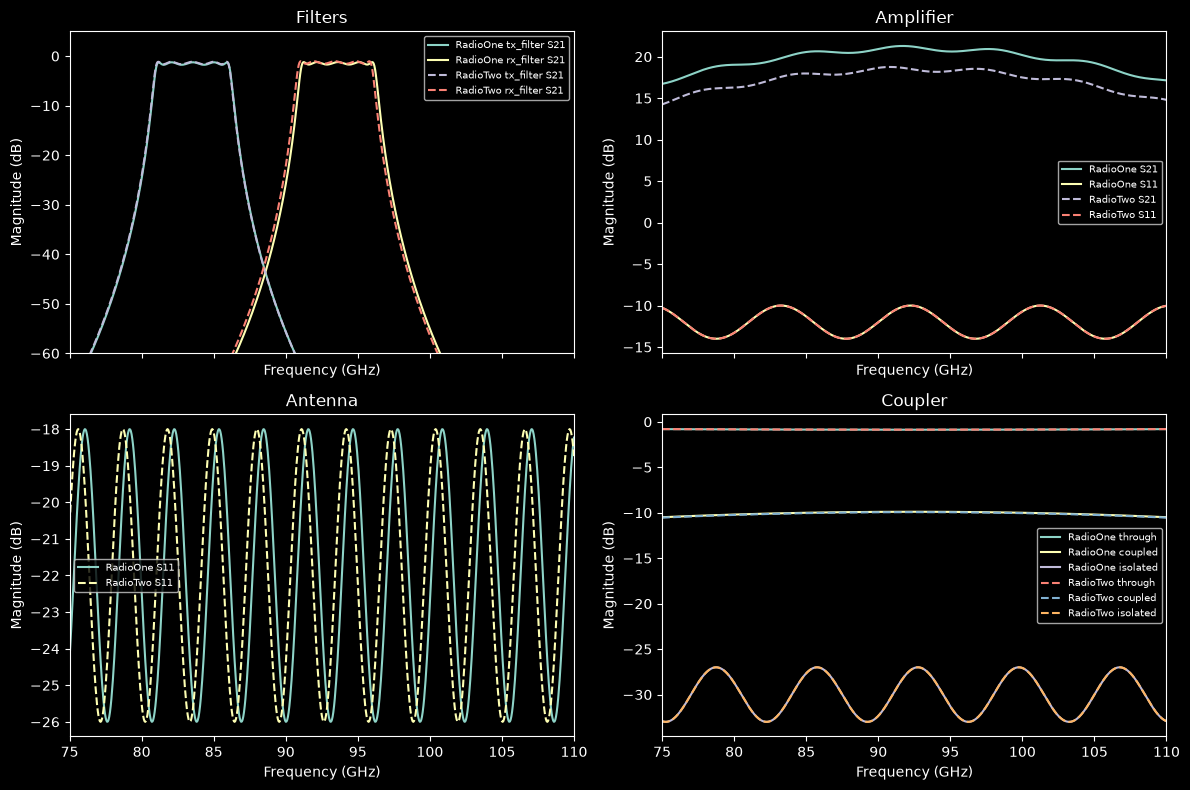
Every part is characterized from 75 to 110 GHz. The radios use frequency-division duplexing: they transmit in 81–86 GHz and receive in 91–96 GHz, so each has a bandpass filter for each direction.
Part |
File |
Model |
|---|---|---|
Tx filter |
|
5th-order Chebyshev bandpass, 81–86 GHz |
Rx filter |
|
5th-order Chebyshev bandpass, 91–96 GHz |
Amplifier |
|
about 21 dB gain, rolling off toward the band edges |
Antenna |
|
horn antenna, return loss only |
Coupler |
|
10 dB directional coupler: port 1 in, 2 through, 3 coupled, 4 isolated |
Each radio’s parts vary slightly, from a fixed random seed. RadioTwo was built with a marginal amplifier, about 2.5 dB below RadioOne’s.
The code that synthesizes data is folded. Select Show code cell source to read it.
scikit-rf writes each network to a Touchstone file whose extension matches its port count:
| RadioOne | RadioTwo | |
|---|---|---|
| tx_filter | rf_radio_data/RadioOne/RadioOne_tx_filter.s2p | rf_radio_data/RadioTwo/RadioTwo_tx_filter.s2p |
| rx_filter | rf_radio_data/RadioOne/RadioOne_rx_filter.s2p | rf_radio_data/RadioTwo/RadioTwo_rx_filter.s2p |
| amplifier | rf_radio_data/RadioOne/RadioOne_amplifier.s2p | rf_radio_data/RadioTwo/RadioTwo_amplifier.s2p |
| antenna | rf_radio_data/RadioOne/RadioOne_antenna.s1p | rf_radio_data/RadioTwo/RadioTwo_antenna.s1p |
| coupler | rf_radio_data/RadioOne/RadioOne_coupler.s4p | rf_radio_data/RadioTwo/RadioTwo_coupler.s4p |
# Overlay the two radios' parts: RadioOne solid, RadioTwo dashed.
fig, axes = plt.subplots(2, 2, figsize=(12, 8), sharex=True)
for radio, parts in RADIOS.items():
    style = {"linestyle": "-" if radio == "RadioOne" else "--"}
    for part in ["tx_filter", "rx_filter"]:
        parts[part].plot_s_db(
            m=1, n=0, ax=axes[0, 0], label=f"{radio} {part} S21", **style
        )
    parts["amplifier"].plot_s_db(
        m=1, n=0, ax=axes[0, 1], label=f"{radio} S21", **style
    )
    parts["amplifier"].plot_s_db(
        m=0, n=0, ax=axes[0, 1], label=f"{radio} S11", **style
    )
    parts["antenna"].plot_s_db(
        m=0, n=0, ax=axes[1, 0], label=f"{radio} S11", **style
    )
    for m, port in [(1, "through"), (2, "coupled"), (3, "isolated")]:
        parts["coupler"].plot_s_db(
            m=m, n=0, ax=axes[1, 1], label=f"{radio} {port}", **style
        )
axes[0, 0].set_ylim(-60, 5)
for ax, title in zip(
    axes.flat, ["Filters", "Amplifier", "Antenna", "Coupler"], strict=True
):
    ax.set_title(title)
    ax.legend(fontsize=7)
fig.tight_layout()
Register the radios as assets#
A few key figures become asset properties, so they show on each asset’s page in Nominal and can be searched. Filter loss is read at the center of each filter’s band, and the rest at the center of the receive band, 93.5 GHz.
def db_at(network: rf.Network, m: int, n: int, ghz: float) -> float:
    return round(float(network.s_db[np.argmin(np.abs(F_GHZ - ghz)), m, n]), 2)


def key_figures(parts: dict[str, rf.Network]) -> dict[str, float]:
    return {
        "tx_filter_insertion_loss_db": -db_at(parts["tx_filter"], 1, 0, 83.5),
        "rx_filter_insertion_loss_db": -db_at(parts["rx_filter"], 1, 0, 93.5),
        "amplifier_gain_db": db_at(parts["amplifier"], 1, 0, 93.5),
        "antenna_return_loss_db": -db_at(parts["antenna"], 0, 0, 93.5),
        "coupler_coupling_db": -db_at(parts["coupler"], 2, 0, 93.5),
    }


pd.DataFrame({radio: key_figures(parts) for radio, parts in RADIOS.items()})
| RadioOne | RadioTwo | |
|---|---|---|
| tx_filter_insertion_loss_db | 1.26 | 1.14 |
| rx_filter_insertion_loss_db | 1.24 | 1.05 |
| amplifier_gain_db | 20.91 | 18.21 |
| antenna_return_loss_db | 24.86 | 21.36 |
| coupler_coupling_db | 9.89 | 9.94 |
NominalClient.get_or_create_asset_by_properties finds each radio by its
properties, or registers it the first time. The example property keeps these assets apart from
real radios with the same radio_id.
Each Touchstone file is uploaded with create_attachment and added to its radio with
add_attachments.
EXAMPLE = "rf_radio_field_test"
PART_DESCRIPTIONS = {
    "tx_filter": "Tx channel filter, 81–86 GHz",
    "rx_filter": "Rx channel filter, 91–96 GHz",
    "amplifier": "W-band amplifier",
    "antenna": "Horn antenna",
    "coupler": "10 dB directional coupler (1 in, 2 through, 3 coupled, 4 isolated)",
}

assets = {}
for radio, parts in RADIOS.items():
    asset = client.get_or_create_asset_by_properties(
        {"radio_id": radio, "example": EXAMPLE},
        name=radio,
        description="W-band (75–110 GHz) point-to-point radio",
        labels=["w-band", "radio"],
    )
    asset.update(properties={**asset.properties, **key_figures(parts)})

    attachments = [
        client.create_attachment(
            path,
            description=f"{radio} {PART_DESCRIPTIONS[part]}, 75–110 GHz",
            properties={
                "part": part,
                "ports": str(parts[part].nports),
                "radio_id": radio,
            },
            labels=["touchstone", path.suffix.lstrip(".")],
        )
        for part, path in touchstone_files[radio].items()
    ]
    asset.add_attachments(attachments)
    assets[radio] = asset

assets["RadioTwo"]
Asset(rid='ri.scout.cerulean-staging.asset.25755fb1-07f4-0b67-6f52-a8ce2d8d6f16', name='RadioTwo', description='W-band (75–110 GHz) point-to-point radio', properties=mappingproxy({'amplifier_gain_db': 18.21, 'example': 'rf_radio_field_test', 'radio_id': 'RadioTwo', 'rx_filter_insertion_loss_db': 1.05, 'antenna_return_loss_db': 21.36, 'tx_filter_insertion_loss_db': 1.14, 'coupler_coupling_db': 9.94}), labels=('w-band', 'radio'), created_at=1793806344912004000, is_archived=False)Field test#
Simulate the field test#
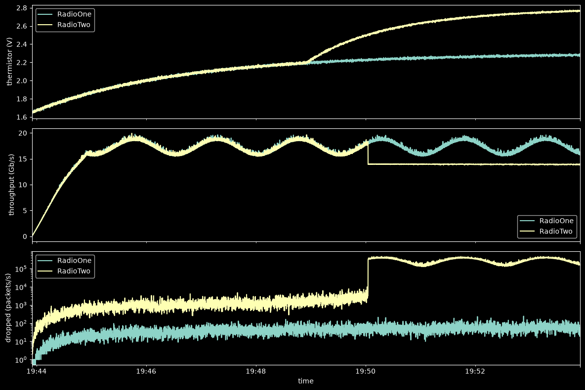
Both radios carry traffic over the same link for 10 minutes, recorded at 10 Hz. Each records:
Dataset |
Channel |
Unit |
What it measures |
|---|---|---|---|
|
|
V |
amplifier drain bias, regulated at 4.0 V |
|
|
V |
12 V supply bus, which sags under load |
|
|
V |
heat: an NTC thermistor divider, which rises as the radio warms |
|
|
million packets/s |
packets received intact |
|
|
packets/s |
packets lost to bit errors or a full queue |
|
|
Gb/s |
delivered throughput |
Traffic is 1500-byte packets, so 1 Mpps is 12 Gb/s. The modem runs at 20 Gb/s, about 1.67 Mpps, while it has at least 2 dB of link margin. Below that, it steps down to a more robust modulation at 14 Gb/s, and back up above 3 dB.
The amplifier loses about 0.05 dB of gain per °C, which eats into the link margin. Five minutes in, RadioTwo’s cooling fan fails. Its marginal amplifier then runs out of margin.
# Plot the simulated test for both radios.
fig, axes = plt.subplots(3, 1, figsize=(12, 8), sharex=True)
for radio, tables in tests.items():
    tables["power"]["thermistor_voltage"].plot(ax=axes[0], label=radio)
    tables["comms"]["throughput_gbps"].plot(ax=axes[1], label=radio)
    tables["comms"]["dropped_packets_pps"].plot(ax=axes[2], label=radio, logy=True)
for ax, label in zip(
    axes, ["thermistor (V)", "throughput (Gb/s)", "dropped (packets/s)"], strict=True
):
    ax.set_ylabel(label)
    ax.legend()
fig.tight_layout()
Upload the field test#
Both radios store their data under the same data scope names, power and comms, so one workbook
template or checklist works for either radio. Asset.get_or_create_dataset
creates each radio’s dataset under its data scope, and upload_dataframe_to_dataset uploads the
test, waiting until Nominal has ingested it.
Then set each channel’s unit and description. The packet-rate channels carry their unit in their names and descriptions.
Each radio’s run also gets its Touchstone files, as a record of the parts the radio had during the test.
CHANNELS = {
    "bias_voltage": ("V", "Amplifier drain bias, regulated at 4.0 V"),
    "dc_supply_voltage": ("V", "12 V supply bus"),
    "thermistor_voltage": (
        "V",
        "NTC thermistor divider from 3.3 V. Rises as the radio warms.",
    ),
    "rx_packets_mpps": (
        None,
        "Packets received intact, in millions of packets per second (1500-byte packets)",
    ),
    "dropped_packets_pps": (
        None,
        "Packets dropped to bit errors or a full queue, in packets per second",
    ),
    "throughput_gbps": ("Gb/s", "Delivered throughput"),
}

runs = {}
for radio, tables in tests.items():
    asset = assets[radio]
    for scope, table in tables.items():
        dataset = asset.get_or_create_dataset(
            scope,
            name=f"{radio} {scope}",
            description=f"{radio} {scope} telemetry from field tests",
            labels=["field-test", scope],
            properties={"sample_rate_hz": SAMPLE_RATE_HZ},
        )
        upload_dataframe_to_dataset(
            dataset,
            table,
            "time",
            "iso_8601",
            file_name=f"{radio}_{scope}_{test_start:%Y%m%dT%H%M%S}.csv.gz",
        )
        for channel in dataset.get_channels():
            unit, description = CHANNELS[channel.name]
            channel.update(unit=unit, description=description)

    runs[radio] = asset.create_run(
        f"{radio} field test {test_start:%Y-%m-%d %H:%M}",
        start=times[0],
        end=times[-1],
        description="10-minute W-band link test at 20 Gb/s line rate",
        properties={
            "site": "Range 4",
            "link_distance_km": 1.2,
            "packet_bytes": 1500,
        },
        labels=["field-test"],
        attachments=asset.list_attachments(),
    )
RadioTwo’s fan failure and the modem stepping down become events, so they show on the timeline in Nominal:
# Look after the first minute, while traffic ramps up and throughput is low anyway.
throughput = tests["RadioTwo"]["comms"]["throughput_gbps"][
    test_start + pd.Timedelta(seconds=60) :
]
first_step_down = throughput[throughput < 15].index[0]
fan_failure = assets["RadioTwo"].create_event(
    "Cooling fan failure",
    EventType.ERROR,
    start=test_start + pd.Timedelta(seconds=300),
    description="Fan tachometer read zero for the rest of the test.",
    labels=["field-test"],
)
step_down = assets["RadioTwo"].create_event(
    "Modem stepped down to 14 Gb/s",
    EventType.FLAG,
    start=first_step_down,
    duration=times[-1] - first_step_down,
    description="Link margin fell below 2 dB. Excess traffic was dropped.",
    labels=["field-test"],
)
Review#
What’s in Nominal#
A card’s name links to its page in Nominal, and its copy button copies its RID.
An asset card lists the asset’s datasets by data scope, its runs and its attachments. Each Touchstone file’s name downloads the file from Nominal, after signing in if needed:
assets["RadioTwo"]
Asset(rid='ri.scout.cerulean-staging.asset.25755fb1-07f4-0b67-6f52-a8ce2d8d6f16', name='RadioTwo', description='W-band (75–110 GHz) point-to-point radio', properties=mappingproxy({'amplifier_gain_db': 18.21, 'example': 'rf_radio_field_test', 'radio_id': 'RadioTwo', 'rx_filter_insertion_loss_db': 1.05, 'antenna_return_loss_db': 21.36, 'tx_filter_insertion_loss_db': 1.14, 'coupler_coupling_db': 9.94}), labels=('w-band', 'radio'), created_at=1793806344912004000, is_archived=False)A run card lists the run’s assets, their datasets and the run’s attachments:
runs["RadioTwo"]
Run(rid='ri.scout.cerulean-staging.run.6e169856-a533-b0da-25cd-fe9410ed4da9', name='RadioTwo field test 2026-11-04 19:43', description='10-minute W-band link test at 20 Gb/s line rate', properties=mappingproxy({'site': 'Range 4', 'link_distance_km': 1.2, 'packet_bytes': 1500.0}), labels=('field-test',), links=(), start=1793821435000000000, end=1793822034900000000, run_number=401, assets=('ri.scout.cerulean-staging.asset.25755fb1-07f4-0b67-6f52-a8ce2d8d6f16',), created_at=1793822120210253000, is_archived=False)A dataset card lists its files and channels:
assets["RadioTwo"].get_dataset("comms")
Dataset(rid='ri.catalog.cerulean-staging.dataset.e5338178-1fa4-1d71-fa01-2749a4f414e6', name='RadioTwo comms', description='RadioTwo comms telemetry from field tests', properties=mappingproxy({'sample_rate_hz': 10.0}), labels=('comms', 'field-test'), bounds=Bounds(start=1793821435000000000, end=1793822034900000000), is_archived=False)A numeric channel’s card shows its statistics and a small chart:
assets["RadioTwo"].get_dataset("power").get_channel("thermistor_voltage")
Channel(name='thermistor_voltage', data_source='ri.catalog.cerulean-staging.dataset.d6e4da43-791d-c583-c5cf-1ae1325fac2b', data_type=<ChannelDataType.DOUBLE: 'DOUBLE'>, unit='V', description='NTC thermistor divider from 3.3 V. Rises as the radio warms.')
An attachment card has a download link for its file:
amplifier_attachments = {
    radio: next(
        a
        for a in asset.list_attachments()
        if a.properties.get("part") == "amplifier"
    )
    for radio, asset in assets.items()
}
amplifier_attachments["RadioTwo"]
Attachment(rid='ri.attachments.cerulean-staging.attachment.cd091a1e-4334-6b65-7ef6-e8084e92f37f', name='RadioTwo_amplifier.s2p', description='RadioTwo W-band amplifier, 75–110 GHz', properties=mappingproxy({'ports': '2', 'radio_id': 'RadioTwo', 'part': 'amplifier'}), labels=('touchstone', 's2p'), created_at=1793822093378029000, is_archived=False)An event card shows the event’s type, start, end and duration:
step_down
Event(rid='ri.scout.cerulean-staging.event.33b1386d-5ddc-2ccf-4384-b51204923e35', asset_rids=('ri.scout.cerulean-staging.asset.25755fb1-07f4-0b67-6f52-a8ce2d8d6f16',), name='Modem stepped down to 14 Gb/s', description='Link margin fell below 2 dB. Excess traffic was dropped.', start=1793821802900000000, duration=232000000000, properties=mappingproxy({}), labels=['field-test'], type=<EventType.FLAG: 'FLAG'>, is_archived=False, disposition=None)Why did RadioTwo drop packets?#
The investigation starts from Nominal, not from the local data. For each radio, find its
field-test run and download the run’s span of the power and comms datasets with
datasource_to_dataframe:
downloaded = {}
for radio, asset in assets.items():
    run = next(r for r in asset.list_runs() if not r.is_archived)
    downloaded[radio] = pd.concat(
        [
            datasource_to_dataframe(
                asset.get_dataset(scope),
                start=run.start,
                end=run.end,
            )
            for scope in ["power", "comms"]
        ],
        axis=1,
    )

pd.DataFrame.from_dict(
    {
        radio: {
            "peak thermistor (V)": data["thermistor_voltage"].max(),
            "mean throughput (Gb/s)": data["throughput_gbps"].mean(),
            "total dropped (packets)": data["dropped_packets_pps"].sum()
            / SAMPLE_RATE_HZ,
            "min bias (V)": data["bias_voltage"].min(),
        }
        for radio, data in downloaded.items()
    },
    orient="index",
).round(3)
| peak thermistor (V) | mean throughput (Gb/s) | total dropped (packets) | min bias (V) | |
|---|---|---|---|---|
| RadioOne | 2.296 | 16.463 | 26244.7 | 3.950 |
| RadioTwo | 2.774 | 15.096 | 68180179.0 | 3.902 |
RadioTwo ran hotter after its fan failed, and throughput fell with it. RadioOne warmed too, but its link held. Plotting dropped packets against the thermistor voltage shows where each radio’s link stopped keeping up:
fig, ax = plt.subplots(figsize=(8, 5))
for radio, data in downloaded.items():
    ax.scatter(
        data["thermistor_voltage"],
        data["dropped_packets_pps"].clip(lower=1),
        s=3,
        label=radio,
    )
ax.set_yscale("log")
ax.set_xlabel("thermistor voltage (V)")
ax.set_ylabel("dropped packets/s")
ax.legend();
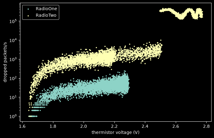
Heat alone doesn’t explain it: at the same thermistor voltage, RadioTwo drops far more packets than RadioOne. Compare the component data. Download each amplifier’s Touchstone file from its attachment, load it into scikit-rf and plot its gain:
downloads = DATA_DIR / "downloaded"
fig, ax = plt.subplots(figsize=(8, 4))
for radio, attachment in amplifier_attachments.items():
    path = downloads / attachment.name
    attachment.write(path)
    rf.Network(str(path)).plot_s_db(m=1, n=0, ax=ax, label=f"{radio} amplifier S21")
ax.axvspan(91, 96, alpha=0.1, label="Rx band")
ax.legend();
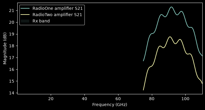
RadioTwo’s amplifier has about 2.5 dB less gain, and its amplifier_gain_db property says so too.
That left it with half the link margin, so the gain it lost to heat after the fan failed pushed it
below the modem’s 2 dB threshold.
Properties make that comparison without downloading anything. search_assets finds both radios,
and their key figures sit side by side:
pd.DataFrame(
    {
        asset.name: dict(asset.properties)
        for asset in client.search_assets(properties={"example": EXAMPLE})
    }
).drop(["example", "radio_id"])
| RadioTwo | RadioOne | |
|---|---|---|
| amplifier_gain_db | 18.21 | 20.91 |
| rx_filter_insertion_loss_db | 1.05 | 1.24 |
| antenna_return_loss_db | 21.36 | 24.86 |
| tx_filter_insertion_loss_db | 1.14 | 1.26 |
| coupler_coupling_db | 9.94 | 9.89 |