

Simulation before hardware#
Story: “I don’t have hardware. I’m building software, test procedures, and simulations, and I may need those results to line up with real tests later.”
This page is for simulation and software engineers who work ahead of hardware, writing models, simulations, and test cases before physical testing starts.
How to organize your data#
To organize test data, start with the simulations approach. In this approach there is a single dataset for each model, and data from each execution is tagged according to what best identifies the data (such as a parameter or an execution ID).
Simulation executions are stored as runs. Upload or stream every execution with the same fixed “zero” timestamp, such as the Unix epoch (1970) or a fixed recent t0, so the executions overlay on top of each other with no shifting.
Executions can keep their real timestamps if desired. In this case, separate time ranges allow you to view each run on a single linear timeline, but to compare them, each run has to be shifted in time.
        ---
config:
  layout: elk

---
flowchart BT
    classDef red fill:#fee2e2,stroke:#b91c1c,color:#1f2937
    classDef purple fill:#e0e7ff,stroke:#4338ca,color:#1f2937

    subgraph dataset1["Dataset: Model A"]
        row1["model=A<br>execution-id=1<br><br>0.0 s · 100.0<br>0.1 s · 101.3<br>..."]:::purple
        row2["model=A<br>execution-id=2<br><br>0.0 s · 100.0<br>0.1 s · 98.7<br>..."]:::purple
    end
    style dataset1 fill:#f5f7ff,stroke:#4338ca,color:#1f2937

    run1["Run A1<br><br>Filters:<br>Model A<br>execution 1"]:::red
    row1 --> run1
    run2["Run A2<br><br>Filters:<br>Model A<br>execution 2"]:::red
    row2 --> run2

    click row1,row2 href "../../../#time-series-data" "Time-series data"
    click run1,run2 href "../../../#runs" "Runs"
Note
If a model is executed thousands of times, such as in a Monte Carlo analysis, it may be challenging to create and use thousands of individual runs. You can instead make a single run which includes all of the data and split it by tag in a workbook. The benefit is you only deal with a single run, but the drawback is that some types of analysis may be harder to perform. For example, Nominal comparison workbooks are built to compare many runs, not data split by tag. See Large campaigns for details on this approach.
If your work is pure simulation, this is all you need. If you expect to have hardware eventually and plan to compare live hardware data against the simulation, you should ensure that each channel’s unique identification is the same. In Nominal, a channel is uniquely identified by its ref name and channel name together, written like default.voltage. If you follow the walkthrough below and use default, make sure the hardware teams use the same ref name. Within the simulation, try to use the channel names the hardware test team uses. As long as the ref names and channel names match, data is straightforward to compare. To align simulation data with real hardware data, see aligning timestamps in a workbook.
When the hardware arrives it can still be organized by either the default approach or the tagged approach. Regardless of approach used for the real hardware, workbooks can be used to compare real and simulated results.
        ---
config:
  layout: elk

---
flowchart BT
    classDef green fill:#dcfce7,stroke:#15803d,color:#1f2937
    classDef red fill:#fee2e2,stroke:#b91c1c,color:#1f2937
    classDef purple fill:#e0e7ff,stroke:#4338ca,color:#1f2937
    classDef blue fill:#e0f2fe,stroke:#0369a1,color:#1f2937

    asset1["Asset: UUT1"]:::green
    dataset1[("UUT1<br>Dataset")]:::purple
    dataset1 -->|"ref name=default"| asset1
    run1["Run: Test A<br>on UUT1"]:::red
    asset1 --> run1

    dataset2[("Simulation<br>Dataset")]:::purple
    run2["Run A7<br><br>Model A<br>execution 7"]:::red
    dataset2 -->|"ref name=default"| run2

    workbook1["Workbook for<br>Model validation<br><br>Looks for `default`.(channel)<br>in each run"]:::blue
    run1 --> workbook1
    run2 --> workbook1

    click asset1 href "../../../#asset" "Asset"
    click dataset1,dataset2 href "../../../#time-series-data" "Time-series data"
    click run1,run2 href "../../../#runs" "Runs"
    click workbook1 href "../../../../workbooks/" "Workbooks"
Walkthrough#
Upload an execution’s output#
Write each execution’s output with timestamps measured from its start, such as the t column of sample-simulation.csv, then upload it with the shared time zero and the execution’s tags.
from datetime import datetime, timedelta, timezone

from nominal import ts
from nominal.core import NominalClient

client = NominalClient.from_profile("default")
dataset = client.get_dataset("<ri.catalog.instance.dataset.identifier>")  # the model's dataset

t0 = datetime(1970, 1, 1, tzinfo=timezone.utc)  # time zero, shared by every execution
tags = {"model": "A", "execution-id": "7"}
file = dataset.add_tabular_data(
    "sample-simulation.csv",
    timestamp_column="t",  # seconds since the execution started
    timestamp_type=ts.Relative("seconds", start=t0),
    tags=tags,
)
file.poll_until_ingestion_completed()  # raises NominalIngestError if the ingest fails
client = nominal.Client.fromProfile();
dataset = client.datasetByRid("<ri.catalog.instance.dataset.identifier>");  % the model's dataset

% Time zero is the Unix epoch, so seconds since the execution started are also epoch seconds
tags = dictionary(["model" "execution-id"], ["A" "7"]);  % "execution-id" can't be a struct field name
client.ingest("sample-simulation.csv", TimestampColumn="t", Kind="epoch", Unit="seconds", ...
    Dataset=dataset, Tags=tags);
use nominal::core::{CsvIngest, TimeUnit, Timestamp};

let client = nominal::NominalClient::from_profile("default")?;
let dataset = "<ri.catalog.instance.dataset.identifier>"; // the model's dataset

let t0 = chrono::DateTime::UNIX_EPOCH; // time zero, shared by every execution
let csv = CsvIngest::new(Timestamp::relative("t", TimeUnit::Seconds).with_offset(t0)) // seconds since the execution started
    .additional_file_tag("model", "A")
    .additional_file_tag("execution-id", "7");
client.ingest().upload_csv("sample-simulation.csv", dataset, csv).await?;
import (
	"bytes"
	"os"

	ingestapi "github.com/nominal-io/nominal-api-go/ingest/api"
	nominalapi "github.com/nominal-io/nominal-api-go/io/nominal/api"
	uploadapi "github.com/nominal-io/nominal-api-go/upload/api"
	"github.com/palantir/conjure-go-runtime/v2/conjure-go-client/httpclient"
	"github.com/palantir/pkg/datetime"
	"github.com/palantir/pkg/rid"
	"github.com/palantir/pkg/safelong"
)

// httpClient is a conjure-go-runtime httpclient.Client for your Nominal REST API URL,
// and token is your API key as a bearertoken.Token
data, _ := os.ReadFile("sample-simulation.csv")
size := safelong.SafeLong(len(data))
path, _ := uploadapi.NewUploadServiceClient(httpClient).UploadFile(ctx, token, "sample-simulation.csv", &size, nil,
	httpclient.RequestBodyInMemory(bytes.NewReader(data)))
datasetRid, _ := rid.ParseRID("<ri.catalog.instance.dataset.identifier>") // the model's dataset

t0, _ := datetime.ParseDateTime("1970-01-01T00:00:00Z") // time zero, shared by every execution
tags := map[nominalapi.TagName]nominalapi.TagValue{"model": "A", "execution-id": "7"}
ingestapi.NewIngestServiceClient(httpClient).Ingest(ctx, token, ingestapi.IngestRequest{
	Options: ingestapi.NewIngestOptionsFromCsv(ingestapi.CsvOpts{
		Source: ingestapi.NewIngestSourceFromS3(ingestapi.S3IngestSource{Path: string(path)}),
		Target: ingestapi.NewDatasetIngestTargetFromExisting(ingestapi.ExistingDatasetIngestDestination{DatasetRid: datasetRid}),
		TimestampMetadata: ingestapi.TimestampMetadata{
			SeriesName: "t", // seconds since the execution started
			TimestampType: ingestapi.NewTimestampTypeFromRelative(ingestapi.RelativeTimestamp{
				TimeUnit: nominalapi.New_TimeUnit(nominalapi.TimeUnit_SECONDS),
				Offset:   &t0,
			}),
		},
		AdditionalFileTags: &tags,
	}),
})
Create a run for the execution#
Create the run over the execution’s time span, with the model’s dataset filtered to the execution’s tags:
run = client.create_run("Model A, execution 7", start=t0, end=t0 + timedelta(seconds=60))
run.add_dataset("default", dataset, series_tags=tags)  # tag filter: only this execution's points
use std::sync::Arc;
use nominal::streaming::api::clients::scout::{AsyncRunService, AsyncRunServiceClient};
use nominal::streaming::api::objects::api::{TagName, TagValue, rids::DatasetRid};
use nominal::streaming::api::objects::scout::{api::DataSourceRefName, run::api::{CreateRunDataSource, CreateRunRequest, DataSource, UtcTimestamp}};
use nominal::streaming::client::{async_conjure_client, conjure::{http::client::{AsyncService, ConjureRuntime}, object::SafeLong}};
use nominal::streaming::prelude::{BearerToken, ResourceIdentifier};

let config = nominal::Config::load()?;
let profile = config.get_profile("default").ok_or("no profile named default")?;
let api = async_conjure_client("runs", profile.base_url().parse()?).map_err(nominal::Error::from)?;
let runs = AsyncRunServiceClient::new(api, &Arc::new(ConjureRuntime::default()));
let source = CreateRunDataSource::builder()
    .data_source(DataSource::Dataset(DatasetRid(ResourceIdentifier::new(dataset)?)))
    .insert_series_tags(TagName("model".into()), TagValue("A".into()))
    .insert_series_tags(TagName("execution-id".into()), TagValue("7".into()))
    .build();
runs.create_run(&BearerToken::new(profile.token())?, &CreateRunRequest::builder()
    .title("Model A, execution 7")
    .description("")
    .start_time(UtcTimestamp::new(SafeLong::new(t0.timestamp())?))
    .end_time(UtcTimestamp::new(SafeLong::new(t0.timestamp() + 60)?))
    .insert_data_sources(DataSourceRefName("default".into()), source)
    .build(),
).await.map_err(nominal::Error::from)?;
Compare executions#
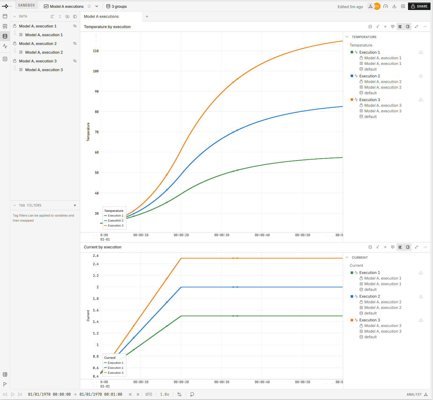
Open a workbook from one execution’s run, add the other runs in its DATA panel (see Line up tests on one timeline), and plot the same channels. Because every execution starts at time zero, the runs overlay as they are. A checklist executed on each run gives every execution its own check results.
Next steps#
Simulations: the full approach, including both extensions.
Repeatable test execution: how to organize the physical tests once the hardware arrives.
🔒︎Automate testing with procedures: if you’re writing test procedures ahead of the hardware too.